MNIST Classification (PyTorch)

0. Overview

본 포스팅에서는 0~9 숫자의 손글씨 이미지를 분류하는 'MNIST Classification'을 PyTorch를 이용해 구현한다. Jupyter Notebook을 이용해 .ipynb 파일에서 코딩을 하였고, 전체 코드는 필자의 github repository를 참고하면 된다. 포스팅에서는 설명을 할 만한 주요 코드 위주로 다루고자 한다.

 

github repository: https://github.com/soohyuncha/MNIST_Classification

GitHub - soohyuncha/MNIST_Classification

구현에 있어 참고한 주요 reference는 다음과 같다.

Reference List

1) Nextjournal

https://nextjournal.com/gkoehler/pytorch-mnist

MNIST Handwritten Digit Recognition in PyTorch

2) Pytorch Github

https://github.com/pytorch/examples/blob/main/mnist/main.py

GitHub - pytorch/examples: A set of examples around pytorch in Vision, Text, Reinforcement Learning, etc.

 

1. Project Setting

1-1. Conda 가상환경 생성 및 활성화

새로운 conda 가상환경을 생성한 뒤, 새로 만든 가상환경인 torch_env를 활성화한다.

conda create -n torch_env python=3.7
conda activate torch_env

1-2. Jupyter notebook 환경 설치

Jupyter notebook을 설치한다.

pip install jupyter notebook
pip install ipykernel

Jupyter notebook에서 가상환경을 사용할 수 있도록 한다. 여기서는 가상환경 이름이 torch_env 이다.

python -m ipykernel install --user --name torch_env --display-name "torch_env"

Jupyter notebook에 들어가보면 다음과 같이 보인다.

참고 링크: https://chancoding.tistory.com/86

Jupyter Notebook에 가상환경 Kernel 연결하기

1-3. 필요한 라이브러리 설치

import torch
import torchvision
import matplotlib.pyplot as plt
import numpy as np

구현에 필요한 라이브러리는 위와 같은데, 만약 import 시 에러가 난다면 다음과 같이 설치한다. 예를 들어, torchvision이 설치되어 있지 않은 경우,

pip install torchvision

 

2. Download Dataset

2-1. Download

torchvision은 여러 dataset을 제공한다. 아래 링크에 들어가보면 torchvision에서 제공하는 데이터셋의 목록을 task 별로 확인할 수 있다. 여기서는 image classification task의 MNIST 데이터셋을 이용한다.

 

링크: https://pytorch.org/vision/stable/datasets.html

Datasets — Torchvision 0.15 documentation

 

데이터셋을 다운로드 받는다.

train_dataset = torchvision.datasets.MNIST('./', train=True, download=True)
test_dataset = torchvision.datasets.MNIST('./', train=False, download=True)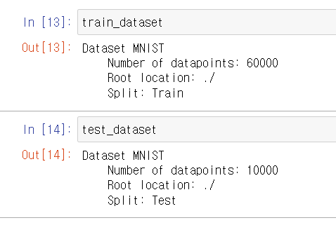

train 데이터 셋은 60,000개, test는 10,000개이다. MNIST 라는 자료형을 가지고 있으며, 인덱싱이 가능하고, 하나의 데이터는 (이미지, 라벨)의 튜플로 되어 있다.

 

그러나 torch의 함수를 이용해 모델을 학습시키기 위해서는 이미지 데이터를 torch의 tensor 형으로 바꾸어주어야 한다. 처음에 다운로드를 받으면 PIL.image 라고 하는 자료형이기 때문에, 다음과 같이 transform argument를 이용해 자료형을 tensor로 바꾼다. 또한 이미지 데이터의 값을 normalize 해주며, train set에 대해 사전에 알려져있는 mean, std 값을 이용한다.

링크: https://discuss.pytorch.org/t/normalization-in-the-mnist-example/457

Normalization in the mnist example

transform=torchvision.transforms.Compose([
        torchvision.transforms.ToTensor(),
        torchvision.transforms.Normalize((0.1307,), (0.3081,))
        ])

train_dataset = torchvision.datasets.MNIST('./', train=True, download=True, transform=transform)
test_dataset = torchvision.datasets.MNIST('./', train=False, download=True, transform=transform)

 

2-2. Display Sample Data

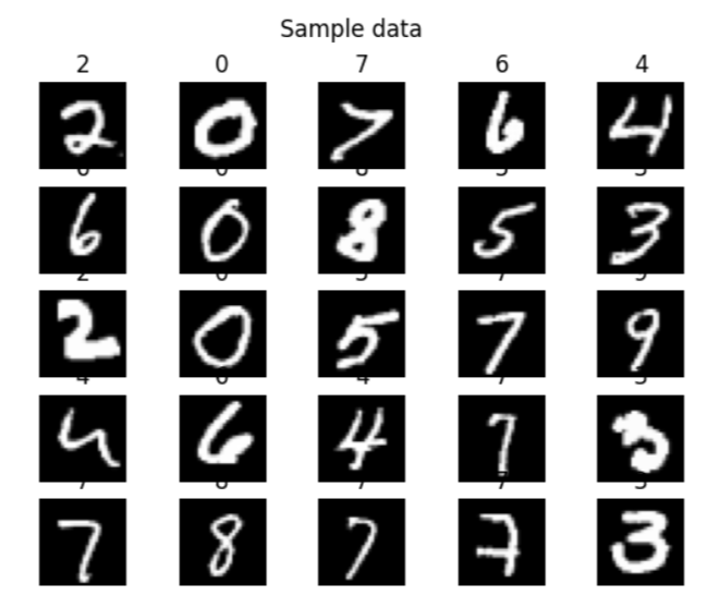
matplotlib의 subplot과 imshow를 이용해 몇 개의 sample train data를 출력해볼 수 있다. 데이터 셋 자료형이 인덱싱이 가능하므로, 튜플을 얻어서 이미지와 라벨로 분류할 수 있다. 다음과 같이 손글씨 이미지와 숫자가 label로 붙어 있다.

 

2-3. DataLoader

torch에서는 DataLoader라는 자료형을 제공하는데, train, test 시에 데이터셋을 batch 단위로 처리할 수 있도록 해준다. 문법은 직관적이며, 데이터셋 자료형을 넣어주고, batch size를 설정한다. shuffle argument는 train epoch마다 데이터의 순서를 섞어줄지에 대한 True/False 이다.

batch_size = 64

train_loader = torch.utils.data.DataLoader(train_dataset, batch_size=batch_size, shuffle=True)
test_loader = torch.utils.data.DataLoader(test_dataset, batch_size=batch_size, shuffle=True)

DataLoader 자료형 document: https://pytorch.org/docs/stable/data.html#torch.utils.data.DataLoader

torch.utils.data — PyTorch 2.0 documentation

 

3. Neural Network Model

이제 모델을 정의하고, train, test 함수를 정의한다.

3-1. Model Class

torch에서는 nn.Module 이라는 base class를 제공하는데, torch로 구현하는 모든 neural network 모델이 이 base class를 상속하도록 해야 한다. init과 forward 함수를 정의하며, convolution이나 fc와 같은 일반적인 layer들은 모두 이미 정의되어 있어서 dimension, padding 등만 paremeter로 넘겨주면 된다.

class NeuralNet(nn.Module):
    def __init__(self):
        super().__init__()
        self.conv1 = nn.Conv2d(1, 16, kernel_size=3, padding=1)
        self.conv2 = nn.Conv2d(16, 32, kernel_size=3, padding=1)
        self.fc1 = nn.Linear(6272, 128)
        self.fc2 = nn.Linear(128, 10)
    def forward(self, x):
        x = self.conv1(x)
        x = F.relu(x)
        x = self.conv2(x)
        x = F.relu(x)
        x = F.max_pool2d(x, 2)
        x = torch.flatten(x, 1)
        x = self.fc1(x)
        x = F.relu(x)
        x = self.fc2(x)
        output = F.log_softmax(x, dim=1)
        return output

nn.Module 코드 중에 __call__ 에 forward 함수가 할당되어 있다. __call__은 클래스의 객체를 함수처럼 호출할 수 있는 것인데, 아래의 두 줄이 같은 실행 결과를 갖는다는 것이 된다.

fc_layer.forward(x)        # forward() 메소드를 호출
fc_layer(x)                # __call__에 의해 객체 호출

nn.Module 코드: https://github.com/pytorch/pytorch/blob/main/torch/nn/modules/module.py#L366

GitHub - pytorch/pytorch: Tensors and Dynamic neural networks in Python with strong GPU acceleration

사용자가 정의하는 NeuralNet 클래스에서 forward를 overriding 해주면, 객체를 호출할 수 있어서 의미가 직관적이게 코드를 작성할 수 있다.

 

3-2. Train

이제 모델을 훈련시키는 코드를 작성한다.

def train(model, train_loader, optimizer, epoch, log_interval):
    model.train()
    for batch_idx, (data, target) in enumerate(train_loader):
        optimizer.zero_grad()
        output = model(data)
        loss = F.nll_loss(output, target)
        loss.backward()
        optimizer.step()
        
        if batch_idx % log_interval == 0 :
            print('Train Epoch: {} [{}/{} ({:.0f}%)]\tLoss: {:.6f}'.format(
                epoch, batch_idx * len(data), len(train_loader.dataset),
                100. * batch_idx / len(train_loader), loss.item()))

맨 첫 줄에서 model.train()은 nn.Module 내에 정의되어 있는 train을 호출한다. 이제 train 데이터셋의 dataloader를 iteration 하면서, batch 단위로 train을 진행한다. 하나의 batch에 대해 train을 한다는 것은 gradient를 back propagation을 통해 구하고 weight을 업데이트 한다는 것인데, 한 번 하고 나면 계산된 gradient 값을 0으로 다시 설정해주어야 하므로, optimizer.zero_grad()를 실행한다. 아래 포스팅에 설명이 잘 되어 있다.

 

링크: https://velog.io/@kjb0531/zerograd%EC%9D%98-%EC%9D%B4%ED%95%B4

zero_grad()의 이해

현재 모델의 forward path를 통과한 output과 데이터셋의 target에 대해 loss를 계산한다. 처음에 이것을 보고 loss.backward가 어떻게 가능한지가 이해가 되지 않았는데, loss가 얼핏 봐서는 loss function에 의해 계산된 스칼라 값이기 때문에 어떻게 backward path를 알고 계산을 이어간다는지가 명확하지 않기 때문이다. 이에 대해서 아래 링크를 읽어보면, 필요한 설명들이 잘 나와있다.

 

간단히만 설명하자면, nn.Module을 상속하는 NeuralNetwork 클래스를 만들고, 설계하고자 하는 구조에 따라 forward 함수를 작성하면, backward 함수는 자동으로 계산된다. output이 모델의 연산 결과로 나오는 tensor이지만, grad_fn 이라고 하는 속성을 가지고 있으며, 이것은 해당 tensor를 계산했던 함수를 참조한다. 자세한 디테일까지 이해하지는 않았지만, 어쨌든 tensor 자료형에 path 정보를 담고 있기 때문에, loss라는 tensor에 대해 backward를 호출하여 재귀적으로 back propagation을 할 수 있다.

 

링크: https://tutorials.pytorch.kr/beginner/blitz/neural_networks_tutorial.html

신경망(Neural Networks)

https://tutorials.pytorch.kr/beginner/former_torchies/autograd_tutorial_old.html

Autograd

이제 gradient를 구했으므로 optimizer.step을 통해 weight을 업데이트하는데, 여기서 optimizer 클래스는 loss를 어떻게 알고 업데이트를 하는 것인지 다시 의문이 들 수 있다. optimizer 클래스 객체를 처음 만들 때 특정 neural network 객체의 parameter 정보를 넘겨준다. 그리고 이 parameter에도 뭔가 계산된 gradient 정보가 있기 때문에, optimizer.step을 했을 때 모든 weight의 gradient 값을 바탕으로 업데이트할 수 있다.

 

3-3. Test

이제 모델이 test dataset에 대해 어떤 성능을 보이는지에 대한 test 함수 코드를 작성한다.

def test(model, test_loader):
    model.eval()
    test_loss = 0
    correct = 0
    with torch.no_grad():
        for data, target in test_loader:
            output = model(data)
            test_loss += F.nll_loss(output, target, reduction='sum').item()  # sum up batch loss
            pred = output.argmax(dim=1, keepdim=True)  # get the index of the max log-probability
            correct += pred.eq(target.view_as(pred)).sum().item()

    test_loss /= len(test_loader.dataset)

    print('\nTest set: Average loss: {:.4f}, Accuracy: {}/{} ({:.0f}%)\n'.format(
        test_loss, correct, len(test_loader.dataset),
        100. * correct / len(test_loader.dataset)))

여기서 train과 다르게 test(=inference)를 할 것이므로 eval과  no_grad를 호출하는데, 그 의미는 일부 layer를 inference 모드로 바꿔주고, gradient 및 path를 추적하는 autograd를 끄겠다는 뜻이다. 실제로 train과 test에서 각각 output을 출력해보면, train에서는 tensor 끝에 gradient 관련된 뭔가가 붙어있는데, test에서는 tensor만 있다.

링크: https://coffeedjimmy.github.io/pytorch/2019/11/05/pytorch_nograd_vs_train_eval/

Pytorch에서 no_grad()와 eval()의 정확한 차이는 무엇일까?

이제 이미지 데이터를 모델에 넣어서 output tensor를 얻고, argmax를 통해 확률이 최대인 label로 선택한다. 이 값을 target(원래 데이터셋에 주어진 정답 label)과 비교해 일치하는 개수를 correct로 세고, 마지막에 이를 퍼센트로 구해 정확도를 측정하게 된다.

 

3-4. Additional Test: Visualize Wrong Data

추가적으로 모델이 예측에 실패한 데이터를 그려볼 수 있다. pred를 얻는 과정은 test 함수와 같다.

 

이미지를 tensor에서 numpy로 바꿔주고, matplotlib의 imshow 함수를 통해 그린다. 예측이 맞는 경우는 제외하고 틀린 경우에 한하여 plot을 한다.

def visualize_wrong_sample(model, test_loader):
    with torch.no_grad():
        sample_batch = next(iter(test_loader))
        img_batch, label_batch = sample_batch
        output_prob = model(img_batch)
        output_pred = torch.argmax(output_prob, dim=1)

    ##### Plot #####
    row, col = 3, 2
    cnt = 1
    for i in range(len(img_batch)):
        if label_batch[i] == output_pred[i]:
            continue
        
        img = img_batch[i].numpy().reshape(28, 28, -1)
        ans, pred = label_batch[i].item(), output_pred[i].item()
        plt.subplot(row, col, cnt)
        cnt += 1
        plt.imshow(img, cmap='gray')
        plt.title('Ans: ' + str(ans) + ', Prediction: ' + str(pred))
    plt.subplots_adjust(wspace=0.5, hspace=0.5)
    plt.suptitle('Visualize Wrong Samples')
    plt.show()
    
visualize_wrong_sample(myNeuralNet, test_loader)

 

4. Run with Script

이제 정의한 모델 클래스에 대한 객체를 만들고, train, test 함수를 실행해 모델의 학습, 평가를 해본다.

myNeuralNet = NeuralNet()
myOptimizer = torch.optim.Adam(myNeuralNet.parameters())

epochs = 3
for epoch in range(epochs):
    train(myNeuralNet, train_loader, myOptimizer, epoch, log_interval=40)
test(myNeuralNet, test_loader)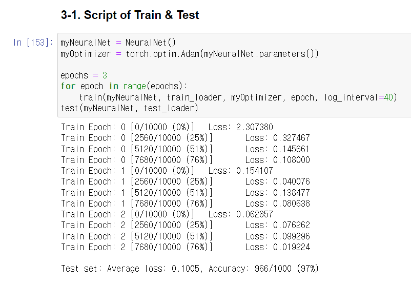

마지막에 test set에 대한 accuracy 결과가 출력된다.

 

예측이 틀린 test 데이터를 확인해볼 수 있다.

visualize_wrong_sample(myNeuralNet, test_loader)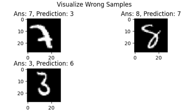

 

5. Save and Load Model

이렇게 train 시킨 모델은 파일로 저장되지 않은 상태이다. 다음에 train 없이 바로 inference 하기 위해서는 모델을 파일로 저장해야 한다. 그러면 이후에 inference를 하고자 할 때 train 없이 파일을 바로 불러올 수 있게 된다.

 

모델에 대한 weight parameter 정보를 다음과 같이 확인할 수 있다.

# 모델의 state_dict 출력
print("Model's state_dict:")
for param_tensor in myNeuralNet.state_dict():
    print(param_tensor, "\t", myNeuralNet.state_dict()[param_tensor].size())
    #print(myNeuralNet.state_dict()[param_tensor])

각각의 param_tensor는 하나의 layer에 해당되고, 이를 key로 하여 state_dict의 값을 확인해보면 학습된 weight 값이 tensor 형태로 들어 있다. 이제 이 정보를 저장해주면 된다.

 

model_path = './CNN_MNIST_Classifier_0618'
torch.save(myNeuralNet.state_dict(), model_path)

 

모델을 불러올 때는 load_state_dict를 이용하고, 이를 통해 불러온 모델은 학습시킨 모델과 정확히 같은 test 결과를 얻는다.

myNeuralNet_loaded = NeuralNet()
myNeuralNet_loaded.load_state_dict(torch.load(model_path))
myNeuralNet_loaded.eval()
test(myNeuralNet_loaded, test_loader)

 

링크: https://tutorials.pytorch.kr/beginner/saving_loading_models.html

모델 저장하기 & 불러오기